Tricky
In this way, first measuring voltage then measuring current, or first measuring current then voltage, changing the position and range of the meter, as well as removing or inserting the link depending on whether you’re measuring current or voltage, the experiment can be undertaken. Yes, it’s tricky, but we never said it was a doddle, did we? You’ll soon get the hang of it and get some good results.
Now plot your results on the graph of Figure 6.8. My results (correct naturally!) are shown in Table 6.2 and Figure 6.11.
Table 6.2 The results of my own experiment
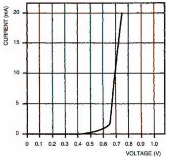
Figure 6.11 My own results from the experiment
Repeat the whole experiment again, using the 0A47 diode, this time. You can put your results in Table 6.3 and plot your graph in Figure 6.12. Our results are in Table 6.4 and Figure 6.13.
Table 6.3 The results of your experiment
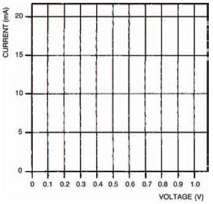
Figure 6.12 Use this graph to plot your results from the second experiment
Table 6.4 My results from the second experiment
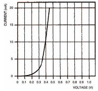
Figure 6.13 A graph plotting my results from the second experiment
As you might expect, these two plotted curves are the same basic shape. The only real difference between them is that they change from a level to an extremely steep line at different positions. The OA47 curve, for example, changes at about 0V3, while the 1N4001 curve changes at about 0V65.
The sharp changes in the curves correspond to what are sometimes called transition voltages — the transition voltage for the OA47 is about 0V3, the transition voltage for the 1N4001 is about 0V65. It’s important to remember, though, that the transition voltages in these curves are only for the particular current range under consideration — 0 to 20 mA in this case. If similar curves are plotted for different current ranges then slightly different transition voltages will be obtained. In any current range, however, the transition voltages won’t be more than about 0.V1 different to the transition voltages we’ve seen here. The two curves — of the OA47 and the 1N4001 diodes — show that a different transition voltage is obtained (0V3 for the OA47, 0V65 for the 1N4001) depending on which semiconductor material a diode is made from. The OA47 diode is made from germanium while the 1N4001 is of silicon construction. All germanium diodes have a transition voltage of about 0V2 to 0V3; similarly all silicon diodes have a transition voltage of about 0V6 to 0V7.
These two curves are exponential curves — in the same way that capacitor charge/discharge curves (see Chapter 4) are exponential, just in a different direction, that’s all — and form part of what are called diode characteristic curves or sometimes simply diode characteristics. But the characteristics we have determined here are really only half the story as far as diodes are concerned. All we have plotted are the forward voltages and resultant forward currents when the diodes are forward biased. If diodes were perfect this would be all the information we need. But, yes you’ve guessed it, diodes are not perfect — when they are reverse biased so that they have reverse voltages, reverse currents flow. So, to get a true picture of diode operation we have to extend the characteristic curves to include reverse biased conditions.
Reverse biasing a diode means that its anode is more negative with respect to its cathode. So by interpolating the xand y-axes of the graph, we can provide a grid from the diode characteristic which allows it to be drawn in both forward and reverse biased conditions.
It wouldn’t be possible for you to plot the reverse biased conditions, for an ordinary diode, the way you did the forward biased experiment (we will, however, do it for a special type of diode soon), so instead we’ll make it easy for you and give you the whole characteristic curve. Whatever type of diode, it will follow a similar curve to that of Figure 6.14, where the important points are marked.
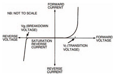
Figure 6.14 Plotting the reverse bias characteristics for an ordinary diode is not practical, so we give you the characteristic curve here
<< Which way round?